Some Secrets Shared

In cryptography, secret sharing is the process of splitting a secret into pieces, called secret shares, so that no individual device stores the original secret, but some group of devices can collectively recover that secret. Classic examples of situations involving secret sharing include missile launch codes and shared custody in the corporate setting; in both cases, multiple individuals’ authorizations are required before any action can be taken. Recently, secret sharing has seen extensive use within multi-party computation (MPC) involving secret data, and private key management, where an individual or organization has cryptocurrency belonging to a secret key and they wish to split this key into \(n\) key shares such that some subset of \(t\) shares is required for using the key.

In this post, we will be discussing two forms of secret sharing: Replicated Secret Sharing (RSS) and Shamir Secret Sharing (SSS). We will introduce the details of both of these schemes assuming relatively little background. We will also introduce a process for converting RSS shares into SSS shares that can be employed to construct a scheme known as Pseudorandom Secret Sharing (PSS) in which a single setup leads to an arbitrary number of secure deterministic SSS instantiations. Finally, we will see these constructions in action in the threshold Schnorr signature scheme, Arctic.

Table of Contents

• 2-of-3 Secret Sharing Examples
• Shamir Secret Sharing
• Lagrange Interpolation
  • Uniqueness of Polynomial Interpolation
• Replicated Secret Sharing
• Pseudorandom Secret Sharing
• Distributed Key Generation
• Recovery in the Exponent
• Verifiable Pseudorandom Secret Sharing
  • A Note on Computing \(\Lambda_{j,k}^C\)
• Application to Threshold Schnorr Signatures
• Conclusion

2-of-3 Secret Sharing Examples

Suppose we wish to split a secret, \(s\), into \(n=3\) pieces, \((s_1, s_2, s_3)\) such that any \(t=2\) secret shares can be used to recover the original secret. For clarity and simplicity, say that we wish to distribute secret shares to three parties, Alice (A), Bob (B), and Carol (C).

One approach is to begin by splitting up the secret into three shares that add up to \(s\). For example, we could pick \(s_1\) and \(s_2\) randomly and then set \(s_3 = s - s_1 - s_2\). This gives us three secret shares such that all three are required to recover our secret; knowing any two secret shares yields no information about \(s\) since it is still equally likely to be any number. Next, we can turn this \(t=3\) scheme into a \(t=2\) scheme by making our secret shares collections of these pieces. Namely, we give Alice the set \(\{s_2, s_3\},\) we give Bob the set \(\{s_1, s_3\},\) and we give Carol the set \(\{s_1, s_2\}\). No individual has any information about \(s\), but if any two of them collaborate, they will collectively know all three summands!

An alternative approach is to use the fact that any two points define an entire line. Thus, if we work in the standard 2-dimensional plane and pick one point to be \((0, s)\), and we pick a second point to have a random second coordinate, \((1, s_1)\), then these two points uniquely define a line which must contain further points \((2, s_2)\) and \((3, s_3)\) for some values of \(s_2\) and \(s_3\). Once we have chosen \(s_1\) at random, there are even nice formulas for our other values that can be derived using very elementary means. For example, we know the slope of this line is \(\frac{s_1 - s}{1 - 0} = s_1 - s\) so that

and

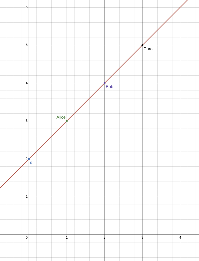
Hence, if we give \((1, s_1)\) to Alice, \((2, s_2)\) to Bob, and \((3, s_3)\) to Carol, then any two of them will be able to collaborate to compute the line going through their two points, and will be able to discover \(s\) by computing the value of the second coordinate when the first coordinate is equal to \(0\). Furthermore, no individual participant has any information at all about the value of \(s\).

Notice that in either method of splitting up our secret, we have the following nice properties:

• If everyone multiplies their secret share by some constant \(c\), then the result is that everyone has a share for \(c\) times the original secret value.
• If we perform the secret sharing twice using the same indices for two different secrets, \(s_1\) and \(s_2\), and if each participant adds their secret shares together, then the result is that everyone has a share for the sum of the secrets, \(s_1 + s_2\).

Together, these properties are referred to as “linearity.”

The linearity of our first method is very easy to see, because each party simply holds a pair of summands that we add together, and clearly,

The linearity of our second method (using lines) is only slightly harder to see. The key idea is that each line can be represented by an equation \(y = L(x)\) for some function \(L\) such that \(L(0) = s\), and our shares \(s_1, s_2, s_3\) are equal to the evaluations \(L(1), L(2), L(3)\). Therefore, if we have two lines \(y = L_1(x)\) and \(y = L_2(x)\) such that \(s = L_1(0)\) and \(s' = L_2(0)\), then the line \(y = L_1(x) + L_2(x) = (L_1 + L_2)(x)\) satisfies \((L_1 + L_2)(0) = s + s'\) and \((L_1 + L_2)(i) = L_1(i) + L_2(i)\) for each \(i=1,2,3\). Here, I’m thinking of \(L_1 + L_2\) as a single new function of \(x\). For example, if \(L_1(x) = 2+x\) as above and \(L_2(x) = 3-5x\), then \((L_1 + L_2)(x) = 5 - 4x\).

Linearity is what enables parties to perform multi-party computations on secret inputs without revealing those secrets. For example, if we have performed secret sharing on a secret key, \(x\), and a secret random nonce value, \(k\), we may wish to compute the value \(s = k + H(R, m)\cdot x\), for some publicly known constant \(H(R, m)\). The value \(s\) is a Schnorr signature of the message \(m\) by the shared key \(x\). Linearity of our secret sharing schemes means that since we have split \(x\) and \(k\) into many pieces in a consistent manner, we can have each participant add \(H(R, m)\) times their share of \(x\) to their share of \(k\) and the result is a share of \(s\). Lastly, the parties can recover \(s\) without having revealed \(k\) or \(x\) at any intermediate step! This means that if we can linearly secret share a value in a 2-of-3 fashion, we can also do many computations on the shared secrets requiring the collaboration of only 2-of-3 of the parties without ever having any single party learn the secret inputs to the computation. We will discuss this use of secret sharing more in depth at the end of this post.

Shamir Secret Sharing

Using lines, as in our example above, works great for any scheme where \(t=2\) meaning that any two participants can compute the secret, but what if you wanted to do something similar to construct a scheme where \(t=3\) participants must collaborate to recover the secret? As it turns out, there is a curve that is uniquely determined by any three of its points: a parabola! (Circles and planes also work, but they don’t generalize as well). More generally, for any number \(t\), a degree \((t-1)\) polynomial is a curve which is uniquely determined by any \(t\) of its points. We justify this claim below. Furthermore, knowledge of any \(t-1\) points yields no information about any other points on the curve assuming that the curve was generated randomly.

In other words, if we want to do a \(t\)-of-\(n\) secret sharing of \(s\), we choose random values \(a_1, a_2,\ldots, a_{t-1}\) and use these to define a polynomial

Because we set the constant term to \(s\), we have that \(f(0) = s\). Next, we set \(s_1 = f(1), s_2 = f(2), \ldots, s_n = f(n)\) and distribute the values \((1,s_1), (2, s_2), \ldots, (n, s_n)\) to their respective parties. Finally, any \(t\) parties can use their shares to reconstruct the polynomial \(f(x)\), because it is determined by any \(t\) of its points, and then they can compute \(s = f(0)\). This scheme is called Shamir Secret Sharing (SSS). But how do we actually compute \(f(x)\) from some set of \(t\) points \((x_1, y_1), (x_2, y_2), \ldots, (x_t, y_t)\)? The problem of computing a curve that fits a given set of points is known as interpolation and is discussed in the next section. For readers already familiar with the details of Lagrange interpolation, skip ahead.

Lagrange Interpolation

Let’s begin with the example of trying to compute a line (where \(t=2\)) given two points: \((x_1, y_1)\) and \((x_2, y_2)\). The slope of our line is \(\frac{y_2 - y_1}{x_2 - x_1}\), and thus we can use the point \((x_1, y_1)\) along with this slope to write down the so-called point-slope form of the line:

However, in its current form, this equation does not generalize particularly nicely to higher degree polynomials, so let us try to rewrite this equation with the goal of having more symmetry between how \(x_1\) and \(x_2\) are used. After all, we could have just as easily used the other point for our point-slope form to get the equivalent line \(y - y_2 = \left(\frac{y_2 - y_1}{x_2 - x_1}\right)(x - x_2).\) As a first step, we isolate \(y\) and separate the \(x\) terms from the \(y_1\)s and \(y_2\)s, and then we distribute and factor out \(y_1\):

The result is a much more symmetric equation that is also relatively easy to understand. If we plug in \(x = x_1\), then we get

Meanwhile, if we plug in \(x = x_2\), then we get

Thus, it appears what is really going on is that we have these “building block” lines, \(L_2(x) = \frac{x - x_1}{x_2 - x_1}\) and \(L_1(x) = \frac{x - x_2}{x_1 - x_2}\), which are equal to either \(0\) or \(1\) when we plug in \(x_1\) or \(x_2\). For example, \(L_2(x_1)\) is equal to \(0\) when we plug in \(x_1\) because the numerator is clearly \(0\), while when we plug in \(x_2\), the denominator of \(L_2(x_2)\) is equal to the numerator, causing the value to be \(1\), and in this case this building block is multiplied by \(y_2\) in the function above so that we get to multiply this \(1\) by \(y_2\) getting us the desired result since \(y = y_2\cdot L_2(x) + y_1\cdot L_1(x).\)

With this example in mind, how might we build similar building blocks for a parabola given three points \((x_1, y_1), (x_2, y_2),\) and \((x_3, y_3)\)? In particular, say that we want to construct a new parabola \(L_1(x)\) such that \(L_1(x_1) = 1, L_1(x_2) = 0\) and \(L_1(x_3) = 0\). To achieve our two \(0\) values, we can begin with the parabola \(y = (x - x_2)(x - x_3)\), and then to ensure that \(L(x_1) = 1\), we can divide this parabola by its current value when \(x_1\) is plugged in giving us

Similarly, we can define \(L_2(x) = \frac{(x - x_1)(x - x_3)}{(x_2 - x_1)(x_2 - x_3)}\) and \(L_3(x) = \frac{(x - x_1)(x - x_2)}{(x_3 - x_1)(x_3 - x_2)}.\) Finally, we can define our parabola

That sure is a mouthful! And it is only going to keep getting bigger, so let’s introduce some notation to make things more compact. Suppose we have a set of participant indices, \(C = \{x_1, x_2, x_3\}\), then for a fixed number \(i\), the building block \(L_i(x)\) that is \(1\) at \(x_i\) and \(0\) for the other values in \(C\) can be described using the following product notation:

In other words, for every \(x_j\in C\) that is not \(x_i\), we multiply in a factor of \(\frac{x - x_j}{x_i - x_j}\). Next, we can concisely write \(f(x)\) using the summation notation:

This notation simply reads that for every value of \(i\) from \(1\) to \(3\), we add in a summand of the form \(y_i\cdot L_i(x)\) for that value of \(i\). In total, we can now write

This final form of \(f(x)\) is finally something that we can generalize to arbitrary degree polynomials. If we are given \(t\) points \((x_1, y_1),\ldots, (x_t, y_t)\) then we can compute the unique degree \(t-1\) polynomial that goes through these points as

where \(C = \{x_1,\ldots, x_t\}\) is the set of \(x\)-coordinates/participant indices. This polynomial goes through the point \((x_k, y_k)\) for every \(k\) because if we plug in \(x_k\) for \(x\), all but one of the summands is equal to \(0\) (because of the \(x - x_k\) factor in the numerator), and the only summand that does not equal \(0\) is the one corresponding to when \(i = k\), in which case the product is equal to \(1\) so that \(f(x_k) = y_k\cdot 1\).

This particular method of reconstructing a polynomial from its points is known as Lagrange interpolation and the “building blocks” that we used, \(L_i(x)\), are known as Lagrange polynomials.

Uniqueness of Polynomial Interpolation

While it is completely sufficient for all practical purposes to simply assume/believe/trust that \(t\) points uniquely define a degree \((t-1)\) polynomial, most arguments for why this must be the case are not particularly difficult (though they can be a bit dense), so I’ve included one such argument here just for fun. No content from this section is required to read the rest of this post.

We wish to prove the claim that if \(f(x)\) and \(g(x)\) are two polynomials of degree \(t-1\), and \(f(x_i) = g(x_i)\) for \(t\) distinct values of \(x_i\), then \(f(x) = g(x)\) as polynomials. The difference of two polynomials of degree \((t-1)\) is of degree at most \((t-1)\), so that \(h(x) = f(x) - g(x)\) is a polynomial of degree at most \((t-1)\) such that its output is \(0\) when evaluated at any of the \(t\) input values \(x_i\). Such an input that causes a function to evaluate to zero is called a root of that function. Therefore, it is sufficient to prove that if a degree \((t-1)\) polynomial, \(h(x)\), has \(t\) distinct roots, then \(h(x) = 0\) (in our case this would imply that \(f(x) - g(x) = 0\Rightarrow f(x) = g(x)\)).

Equivalently, we can show that if \(h(x)\) is a non-zero polynomial of degree at most \((t-1)\), then it can have at most \((t-1)\) roots (as this implies that having more roots makes \(h(x)\) into the zero function). If \(t = 1\), then \(h(x)\) is a polynomial of degree at most \(t-1 = 1-1 = 0\) so that \(h(x)\) is a constant non-zero value and thus it has no roots (since we are assuming that \(h(x)\) is not the \(0\) function). If \(t = 2\), then \(h(x)\) is of degree at most \(t-1 = 2-1 = 1\) making it a non-zero line or a non-zero constant function, both of which have at most \(1\) root. We now continue our argument using induction. (If you aren’t familiar with induction but are familiar with recursion in programming, it is essentially the name for recursion when used in a formal argument such as this one).

Suppose every non-zero polynomial of degree at most \((n-1)\) has at most \((n-1)\) roots; we wish to show that this implies that every non-zero polynomial of degree \(n\) has at most \(n\) roots. Let \(h(x)\) be an arbitrary non-zero degree \(n\) polynomial. If \(h(x)\) has no roots, then it has fewer than \(n\) roots and we are done. Otherwise, there is some value \(a\) such that \(h(a) = 0\). Consider the polynomial, \(p(x) = h(x + a)\), that is the result of plugging in \((x+a)\) for \(x\). This is a new polynomial of degree at most \(n\). Furthermore, we have that \(p(0) = h(0 + a) = h(a) = 0\) from which we can conclude that every term of \(p(x)\) (in its expanded form) is divisible by \(x\) so that we can factor this out to get that \(p(x) = x\cdot q(x)\) for some polynomial \(q(x)\) of degree at most \((n-1)\). Finally, we can use the fact that

to see that \(h(x)\) is equal to \((x-a)\) times a polynomial of degree at most \((n-1)\), which must have at most \((n-1)\) roots by our inductive hypothesis, so that we can conclude that \(h(x)\) has at most \(n\) roots, as desired.

To summarize, we have shown that if a polynomial, \(h(x)\), has a root, \(a\), then \(h(x) = (x-a)\cdot q(x)\) for some polynomial, \(q(x)\), of lesser degree; hence, by induction, it is clear to see that all non-zero polynomials of degree at most \((t-1)\) have at most \((t-1)\) roots, and thus if \(h(x) = f(x) - g(x)\) has \(t\) roots (since \(f(x)\) and \(g(x)\) agree on \(t\) distinct values), we can conclude that \(h(x) = f(x) - g(x) = 0\Rightarrow f(x) = g(x)\).

Replicated Secret Sharing

Recall from our 2-of-3 example at the beginning of this post that there is another way to construct a secret sharing scheme by creating a set of additive secrets, which are random subject to the constraint that the sum of all of the additive secrets is the original secret value, and then sharing some subset of these secrets with each participant in such a way that any \(t\) of them collectively know all of the secrets. This idea can be formalized and generalized in the following way:

For each subset \(a_i\subseteq \{1,2,\ldots, n\}\) of size \(t-1\), create a secret value \(\phi_i\), where all but one of these values is chosen randomly and the final value is chosen so that the sum of all of the \(\phi_i\) is equal to the secret, \(s\). Share the value \((\phi_i, a_i)\) with each member whose index is not in \(a_i\). In other words, for every “maximally unqualified subset” of participants, which are the subsets of size \(t-1\), create a secret known to everyone not in that group of \(t-1\) participants. This guarantees that \(t\) participants are required to recover the secret as any \(t-1\) participants collectively do not know one of the secrets. Furthermore, every \(t\) participants do collectively know all of the secrets, since at least one of the \(t\) must be in the complement of any subset \(a_i\) of size \(t-1\).

For example, say that you wanted to perform a \(3\)-of-\(4\) secret sharing between Alice (\(1\)), Bob (\(2\)), Carol (\(3\)), and Dave (\(4\)). Then we begin by enumerating all of the subsets of \(\{1,2,3,4\}\) of size \(3-1=2\):

Next, we compute \(6\) corresponding values \((\phi_1, \phi_2, \phi_3, \phi_4, \phi_5, \phi_6)\) that sum to \(s\) by picking \(\phi_1\) through \(\phi_5\) at random and then setting \(\phi_6 = s - \sum_{i=1}^5\phi_i\). Finally, \((\phi_1, a_1)\) is given to Carol and Dave, \((\phi_2, a_2)\) is given to Bob and Dave, \((\phi_3, a_3)\) is given to Bob and Carol, \((\phi_4, a_4)\) is given to Alice and Dave, \((\phi_5, a_5)\) is given to Alice and Carol, and \((\phi_6, a_6)\) is given to Alice and Bob. In the end, Alice knows \(\{\phi_4, \phi_5, \phi_6\}\), Bob knows \(\{\phi_2, \phi_3, \phi_6\}\), Carol knows \(\{\phi_1, \phi_3, \phi_5\}\), and Dave knows \(\{\phi_1, \phi_2, \phi_4\}\). As a result, any two of them collectively are missing one of the secrets and hence know no information about \(s\), while any three of them collectively know all of the secrets and can recover \(s\).

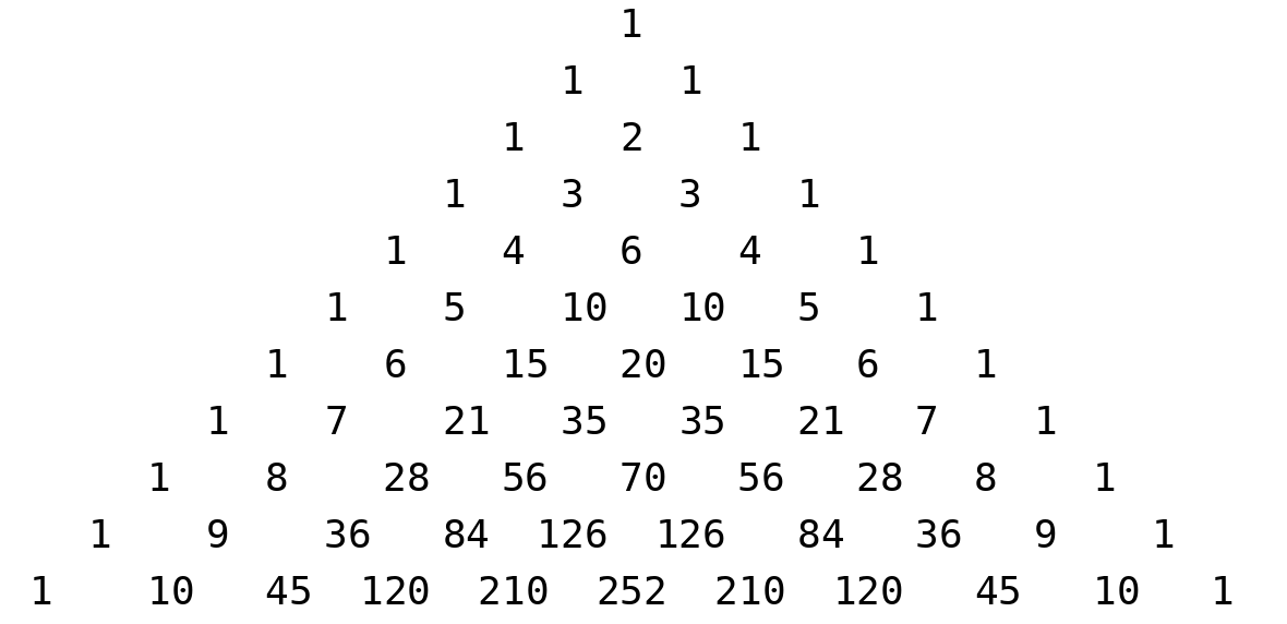
You may notice that while a \(2\)-of-\(3\) replicated secret sharing (RSS) scheme only required \(3\) secret summands, where each participant was given \(2\), our \(3\)-of-\(4\) example required \(6\) secret summands, where each participant was given \(3\). In general, the total number of secret summands in a \(t\)-of-\(n\) RSS scheme is the number of subsets of \(\{1,2,\ldots, n\}\) of size \(t-1\), which is denoted by \(\binom{n}{t-1}\) (pronounced \(n\) “choose” \(t-1\)), and each participant receives each summand corresponding to a subset of size \(t-1\) not containing themselves, of which there are \(\binom{n-1}{t-1}\). This is somewhat grave news for RSS, especially compared to SSS above where each party receives a single number. The value of \(\binom{n}{t}\) (depicted below with \(n\) corresponding to rows and \(t\) corresponding to diagonal columns) grows exponentially large with \(n\) unless \(t\) stays bounded or unless \(n-t\) stays bounded (and even in these cases the values still grow large).

Thus, despite the simplicity of RSS, it is no big surprise that SSS has become the default method of secret sharing. However, in many practical applications, such as private key management, the number of devices involved (\(n\)) is relatively small. For example, even if \(10\) devices are used, then in the worst case we require \(\binom{10}{5} = 252\) summands, \(\binom{9}{5} = 126\) of which are known to each device so that if each secret number is \(32\) bytes, then each party only needs to store approximately \(4\) kilobytes of data. Meanwhile, the worst case for \(20\) devices requires each device to store approximately \(3\) megabytes of data. It is clear that RSS scales poorly to large numbers of devices, but it is still perfectly practical to use for relatively small numbers of signers such as these.

Beyond simplicity, another benefit of RSS that we will not focus on in this post is that it enables secret sharing that goes beyond thresholds to more general recovery policies. For example, if there is a secret shared between Alice (A), Bob (B), Carol (C), Dave (D), and Erin (E), where two of A, B, and C should be able to recover the secret, or two of A, D, and E should be able to recover the secret, then we can create \(5\) secret summands such that \(\sum_{i=1}^5\phi_i = s\) and give A \(\{\phi_2, \phi_3, \phi_4, \phi_5\}\), give B \(\{\phi_1, \phi_2, \phi_3\}\), give C \(\{\phi_1, \phi_4, \phi_5\}\), give D \(\{\phi_1, \phi_2, \phi_4\}\), and give E \(\{\phi_1, \phi_3, \phi_5\}\). Since A is missing only \(\phi_1\) and all other parties know this secret, A and any one other party can recover the secret. Furthermore, B and C know all five secrets together as do D and E, and no one of B or C together with one of D or E know all five secrets. This can be generalized to capture any policy, but we will continue to focus on threshold secret sharing for the rest of this post.

Pseudorandom Secret Sharing

One benefit that RSS has, which SSS does not, is that if we are sharing many randomly generated secrets, then rather than setting up a new sharing for each secret we can instead perform a RSS setup a single time and treat each of the secret summands as a key (a.k.a seed) to a pseudorandom function (PRF). Subsequently, we can non-interactively generate an unlimited number of RSS-shared secrets deterministically. Specifically, one way to do this is to fix a cryptographic hash function, \(H\), then given some session identifier, \(sid\), and a secret seed, \(\phi_i\), we can compute the new secret \(\alpha_i = H(\phi_i\vert\vert sid)\). If each party computes \(\alpha_i\) for every \(\phi_i\) that they know, then they can use these new values as their RSS shares of the pseudorandom secret \(s_{sid} = \sum_i \alpha_i\). Notice that no communication is required between the participants to set up this new RSS of the secret \(s_{sid}\)! Each participant only does local computation on values they already have from the initial replicated PRF seed setup. The key point is that because PRFs are deterministic for a fixed seed, parties are able to compute the replicated values \(\alpha_i\) without communicating with one another so long as they know the replicated secret \(\phi_i\).

This kind of scheme is not possible to create based on an initial Shamir Secret Sharing setup because each participant knows a point on a polynomial curve, which cannot be used as a seed for a PRF because the outputs from such a setup will not lie on the same degree \((t-1)\) polynomial. In fact, if each of the \(n\) participants have some PRF that is seeded randomly using any means and without replication, and they treat the outputs of these PRFs as Shamir shares, then with overwhelming probability the points that are output will not lie on any polynomial of degree less than \(n-1\) (where \(n\) is the number of points). The issue is that Shamir shares are correlated because any \(t\) points determine all \(n\) points. This is not a problem for RSS because secret summands are not correlated.

However, the primary downside of RSS when compared to SSS is the storage and communication complexity. In SSS, you only need to keep track of a single secret. Furthermore, when you are using this secret as part of a multi-party computation, such as when you are computing a partial signature, then you only need to compute a single partial signature. Meanwhile, with RSS you may have to compute and communicate the partial signature for every share you know. There is no way to reduce the storage requirements of RSS, but it is possible to convert RSS shares (which are made up of many secret summands) into SSS shares (which are a single secret point) without introducing any communication! This means that for the cost of a single RSS initial setup, you can deterministically generate arbitrarily many pseudorandom SSS-distributed secrets without any further communication by creating RSS secrets and then converting the resulting RSS shares into SSS shares.

The key idea behind converting an RSS-distributed secret into a SSS-distributed secret is that we must define a polynomial, \(f_{sid}(x)\), of degree \((t-1)\) such that \(f_{sid}(0) = s_{sid} = \sum_i \alpha_i = \sum_i H(\phi_i, sid)\) and for every \(k\in\{1,\ldots, n\}\), \(f_{sid}(k)\) is a value that can be computed by participant \(k\), that is, \(f_{sid}(k)\) can be computed using only the secret values \(\phi_i\) that participant \(k\) has access to. Define \(L_{a_i}(x) = \prod_{j\in a_i}\frac{j-x}{j}\), which is the unique degree \(\vert a_i\vert = t-1\) polynomial such that \(L_{a_i}(0) = 1\) and \(L_{a_i}(k) = 0\) for all \(k\in a_i\). If we let

then this is a degree \((t-1)\) polynomial such that

and for every \(k\in\{1,\ldots,n\}\),

Notably, one does not need to know \(\phi_i\) for any \(i\) such that \(k\in a_i\) in order to compute \(f_{sid}(k)\) since \(L_{a_i}(k) = 0\) for all \(i\) such that \(k\in a_i\). Thus, participant \(k\) can compute \(f_{sid}(k)\) locally from only the secrets they know because they know exactly all \(\phi_i\) such that \(k\notin a_i\).

Therefore, after a single RSS setup, we can compute arbitrarily many Shamir secret sharings without any further communication by having each party compute their secret share for session identifier, \(sid\), as \(s_{sid,k} = \sum_{i\text{ with }k\notin a_i} H(\phi_i, sid)\cdot L_{a_i}(k).\) Also note that the values \(L_{a_i}(k) = \prod_{j\in a_i}\frac{j-k}{j}\) do not change between sessions so that they can be cached for efficiency.

This scheme is called Pseudorandom Secret Sharing (PSS) and was first developed by Cramer et al. in this paper in 2004. PSS basically allows protocols to have all the benefits of repeated RSS use with only a single setup and communication complexity that is equivalent to Shamir-based schemes after setup (because of the share conversion). Furthermore, the security of PSS-based schemes tends to be relatively simple to reason about by simulation arguments reducing to pure RSS-based variants (which are inefficient but very simple to reason about). Basically, the security argument usually has three phases:

1. Reduce the security of the PSS-based scheme to the security of that scheme using pure RSS.
2. Reduce the security of the RSS-based scheme to the security of the non-threshold version where all participants’ cooperation is required and the adversary controls all but one participant.
3. Prove the security of the non-threshold version.

For example, this is how Iceberg reduces its security to that of Nested MuSig2 (this paper is in preparation).

Distributed Key Generation

So far we have been discussing the setup of our secret sharing schemes in terms of a trusted dealer who knows the underlying aggregate secret and splits it into shares and deals shares out to participants. In practice, we usually want to replace a trusted dealer with a trustless distributed key generation (DKG) protocol.

DKGs for RSS are extremely simple! For each secret summand, one party who is meant to know that secret (designated in any way, for example, the lowest index party) generates the secret at random and shares it with all other participants who need to know that secret. Then, participants verify that they have all received the same secret. For example, this verification check can be accomplished by having each participant respond to the party that generated the secret with a signature of that secret, and then having the generator collect all of these signatures and send the entire collection to each party for batch verification.

So far in this blog post, we have not discussed any public key cryptography directly, as we have only been discussing secret values with no relation to “public keys.” The remainder of this post is entirely about the relation of our secrets to public keys. In particular, we will assume familiarity with cyclic groups and their use in discrete log-based public key cryptography.

In 1987, Paul Feldman published a verifiable secret sharing (VSS) scheme that allows an untrusted dealer to perform a SSS setup. As in the trusted setup we described above, the dealer chooses a polynomial \(f(x) = s + a_1x + a_2x^2 + \cdots + a_{t-1}x^{t-1},\) where the values \(a_1,\ldots, a_{t-1}\) are chosen uniformly at random, and the dealer distributes the values \(s_i = f(i)\) to participant \(i\). Additionally, the dealer gives every participant the list of values \(P_0 = g^s, P_1 = g^{a_1},\ldots, P_{t-1} = g^{a_{t-1}}\), which are the public keys if we treat the coefficients of \(f(x)\) as private keys. Each participant, \(i\), can then verify their secret share “in the exponent” by checking that

If no party complains that their share is invalid, then the setup is a success. This VSS can be transformed into a DKG by having each participant generate a uniformly random secret, and then act as the dealer to all other participants. The result is that every party holds a Shamir share of every participant’s secret. Assuming that each participant has a fixed index meaning that they know the value of each polynomial at a fixed x-coordinate, then every participant can add up all of their shares and the result is a share on the sum of all of the polynomials, which is itself a polynomial. Essentially, each party generates a secret summand and we let the aggregate DKG secret be the sum of all of these values, then each participant acts as an untrusted dealer for their summand, and finally everyone adds their summand shares together to get a single share for the aggregate secret.

As you may have noticed, SSS DKGs are quite a bit more involved than RSS DKGs, so that if you don’t have too many participants (ensuring RSS is practical) and you need to do many SSS DKGs, it may be preferable to use PSS, which yields arbitrarily many SSS DKGs for the cost of a single RSS DKG.

Recovery in the Exponent

Suppose you have an RSS secret, \(s\), that has already been dealt among some participants (either directly or as the result of Pseudorandom Secret Sharing). Then it is quite simple to compute the public key \(g^s\) without recovering \(s\) by having each party broadcast the public keys of all of their secret summands, verifying that all parties agree, and then taking a product of each (deduplicated) factor. In other words, if

then

Similarly, if \(s\) has been dealt using SSS (either directly or as a result of Pseudorandom Secret Sharing), then so long as all parties not only know their share \(s_i = f(i)\), but also know the public keys \(P_j = g^{s_j}\) for all values \(j\), any \(t\) of them can compute \(g^s\) by using interpolation “in the exponent” like so:

where \(C = \{i_1,\ldots, i_t\}\) and \(\lambda_j = L_{i_j}(0) = \prod_{i_k\in C\setminus\{i_j\}}\frac{i_k}{i_k - i_j}.\)

However, it is not necessarily simple to just “also know the public keys \(P_j\)” because we do not know the underlying private keys (party \(j\)’s share) and we may not trust party \(j\). If Feldman’s VSS-based DKG was used to set up the SSS, then we can compute these values trustlessly from the intermediate commitments. In the next section, we describe how we can verify supposed \(P_j\) values in the context of PSS.

Verifiable Pseudorandom Secret Sharing

For a fixed \(sid\), recall that party \(k\) locally computes its share as

The key idea is that we want to come up with some kind of computation that could be used to check that some set of \(s_k\) values are valid that can be carried out “in the exponent.” Namely, if we are given the values \(s_{i_1},\ldots, s_{i_{2t-1}}\) that are allegedly equal to \(f(i_1),\ldots, f(i_{2t-1})\), then we should be able to use interpolation to compute \(f\) from these values. In particular, we can check the degree of \(f\), which should be equal to \(t-1\).

If we assume that there are at most \(t-1\) dishonest parties, so that there is an honest majority, then any collection of at least \(2t-1\) participants contains at least \(t\) honest participants. This means that we can recover the true value of \(f\) through interpolation from these parties alone. But what happens if we add more points to our interpolation? If those points are correctly computed, i.e., \(s_i = f(i)\), then the interpolation will still output the same polynomial \(f\). However, if a dishonest party uses a value \(s_i\neq f(i)\), then interpolation of honest points alongside the point \((i, s_i)\) will result in a polynomial of degree higher than \(t-1\). This is because \(f\) is the unique degree \((t-1)\) polynomial going through the \(t\) honest points, and adding any points not on that polynomial requires interpolation through more than \(t\) points and will result in a higher-degree polynomial. Therefore, if we make an honest majority assumption, then computing the degree of the polynomial interpolated through at least \(2t-1\) shares is sufficient to verify the correctness of those shares. Note that interpolating using \(m\geq 2t-1\) points results in a polynomial of degree at most \(m-1\), and we are simply verifying that the coefficients on \(x^t, x^{t+1}, \ldots, x^{m-1}\) are all \(0\).

Now we translate this computation “to the exponent.” Given a set of values \(\{D_j\}_{j\in C}\) such that \(D_j\) is supposedly equal to \(g^{s_j}\), where \(s_j = f(j)\), we want to compute \(g^{f(x)} = g^{\sum_{j\in C}s_j\cdot L_{C, j}(x)}\), where \(L_{C,j}(x) = \prod_{i\in C\setminus\{j\}}\frac{i-x}{i-j}\). If we use \(\Lambda_{j,k}^C\) to denote the degree \(k\) coefficient of \(L_{C,j}(x)\) when it is expanded so that

then we can collect like terms to get

Therefore, if we let \(f(x)\) be the result of interpolating using the values \(\{s_j\}_{j\in C}\), then

is the result of “interpolating in the exponent” using \(\{D_j\}_{j\in C}\). Therefore, in the honest-majority setting, it is sufficient to verify that \(\prod_{j\in C}D_j^{\Lambda_{j,k}^C} = g^0 = \text{Id}_{\mathbb{G}}\) for all \(k\geq t\). If this is the case, then all of the values \(\{D_j\}_{j\in C}\) must be the public keys of secrets lying on the same degree \(t-1\) polynomial, which must be the correct polynomial by the honest majority assumption (which guarantees that at least \(t\) of the inputs to interpolation are honest).

Thus, in the honest-majority setting, we now have Verifiable Pseudorandom Secret Sharing (VPSS)! With VPSS we can not only get infinite free SSS secrets from a single RSS DKG, but we can also verify participant shares and thus we can verifiably compute the aggregate public keys (i.e., perform recovery in the exponent) for the underlying distributed secrets without recovering those secrets directly.

Note that it is possible to have alternate verification using zero-knowledge proofs (ZKPs), which would not require an honest majority assumption. For example, if the VPSS setup (which is an RSS DKG) ends with everyone knowing the public keys of all of the secret pseudorandom function seeds, then participants can generate ZKPs that their point, \(D_j\), was computed correctly. To make such proofs practical, using algebraic hash functions such as MiMC to define the pseudorandom function may be necessary.

A Note on Computing \(\Lambda_{j,k}^C\)

If you aren’t interested in the details of optimal ways to compute \(\Lambda_{j,k}^C\), feel free to skip ahead.

The degree of \(L_{C,j}(x)\) (i.e., the number of values of \(k\)) is equal to \(\vert C\vert\), and there are also that many values of \(j\), so there are \(\vert C\vert^2\) total values to compute. We can expand each of \(L_{C, j}(x) = \prod_{i\in C\setminus\{j\}}\frac{i-x}{i-j}\), but doing so naively takes \(O(\vert C\vert^3)\) time. However, it is clearly possible to do better, since we can rewrite \(L_{C,j}(x) = \frac{A_{C,j}(x)}{A_{C,j}(j)},\) where \(A_{C, j}(x) = \prod_{i\in C\setminus\{j\}} i - x = \frac{A_C(x)}{j-x}\), where \(A_C(x) = \prod_{i\in C}i-x\). We can compute \(A_C(x)\) in \(O(\vert C\vert^2)\) time and then use Horner’s method both to compute \(A_{C,j}(x)\) and to evaluate \(A_{C,j}(j)\) in time \(O(\vert C\vert)\), and we need to do this second part \(\vert C\vert\) times yielding a total result that takes only \(O(\vert C\vert^2)\) time (which is optimal considering the number of values we are computing). This procedure is a variant of the more optimized Parker-Traub algorithm.

There are other methods for efficiently computing the values \(\Lambda_{j,k}^C\), however. Most efficient algorithms for computing these values use the observations that if \(C = \{i_1, i_2, \ldots, i_n\}\), then since \(L_{C, i_j}(i_\ell)\) is equal to \(1\) if \(\ell = j\) and \(0\) otherwise, and that \(L_{C, i_j}(x) = \sum_{k=0}^{\vert C\vert - 1}\Lambda_{j,k}^Cx^k\). Hence, we get the following product of matrices:

Therefore, we can conclude that the matrix containing all of the values \(\Lambda_{j,k}^C\) that we are interested in computing is the inverse of the square Vandermonde matrix generated by \(C\). In other words, the matrix containing all of the values we wish to compute happens to be the inverse to a very highly structured matrix whose inversion can be efficiently computed.

The Bjorck-Pereyra algorithm decomposes a Vandermonde matrix into the product of structured sparse matrices, enabling fast \(O(n^2)\) inversion of that matrix and yielding another efficient method for computing the values we need to perform verification.

The Vandermonde Matrix Inversion Efficiency Algorithm (VIMEA) is an alternative approach that uses recursive computation on elementary symmetric polynomials to compute the inverse matrix in a largely division-free way, making it the most-likely best candidate when working over \(\mathbb{F}_p\) as we are.

Application to Threshold Schnorr Signatures

To close out this post, let’s zoom out and briefly consider the design space for Schnorr threshold signatures in light of all that we have learned in this blog post. I plan to write a more detailed deep-dive into Schnorr threshold signatures in the future, but here’s a teaser. For background on what a Schnorr signature is, see this previous post. For background on the usefulness of Schnorr threshold signatures, see this previous post. To understand this section, it will be important to understand the role a private key and a nonce play in a Schnorr signature.

FROST, which we have discussed in a previous post, is a round-optimized protocol that allows a group of participants that have a SSS-distributed private key to perform the multi-party computation resulting in a Schnorr signature for their shared private key. FROST is so well known that in many circles, people use the term FROST when they actually just mean “Schnorr threshold signature scheme.” However, there are plenty of other threshold signature schemes for Schnorr other than FROST out there, and each has its own trade-offs.

One such alternative, which is also a 2-round protocol, is called Arctic (see Figure 6 on page 20). Arctic also applies to a SSS-distributed private key, but uses VPSS to generate shared nonce values. (In fact, the framework of verifiability in VPSS was originally introduced by Arctic). In contrast, FROST delays the determination of the aggregate nonce to the second round of signing, at which point the subset of parties that will be collaborating to generate the signature is known, and FROST simply additively combines contributions from each of these parties. This difference gives Arctic three important benefits over FROST:

1. The aggregate nonce is determined and known after the first round, before signing session participants are chosen. This property is essential when trying to nest a two-round signing protocol within another two-round signature scheme such as MuSig2 or recursively within itself. (See the Nested MuSig2 paper for an introduction to nesting signature schemes).
2. Arctic does not introduce sensitive state beyond the initial key generation setup because all VPSS outputs can be deterministically re-computed. (FROST requires a new secret nonce contribution to be stored for each signing session).
3. Arctic provides fully deterministic functionality after the initial key generation setup. In many contexts, this makes it possible to make it much harder for an attacker to cause a nonce re-use.

On the other hand, the primary drawbacks of Arctic compared to FROST are:

1. Due to the PSS/RSS setup, Arctic does not scale to very large sets of signers (e.g., more than 20).
2. Arctic requires an honest majority assumption.

However, this second point is a little misleading because firstly, it is possible to replace VPSS verification with ZKPs to remove the honest-majority requirement, and secondly, there is actually a variant of Arctic that uses PSS without using verification at all that does not require an honest majority (I am working on writing up this variant and its security proof). Thus, the primary trade-off to consider here is between the three benefits listed above and the size of state and computation explosion when large numbers of signers are involved. Therefore, since most applications of threshold signatures use fewer than 10 total signers, I personally believe that FROST is usually an inferior threshold signature scheme for most use-cases when compared to PSS-based threshold signatures (such as variants of Arctic), especially in protocols that have well-defined signing session identifiers.

Conclusion

In this post, we have introduced Shamir Secret Sharing and Replicated Secret Sharing, as well as the mathematical tools that power them and methods for Distributed Key Generation. We discussed why SSS is the preferred general secret sharing tool, but we also discussed how there are still many applications that would be better off using (Verifiable) Pseudorandom Secret Sharing (V)PSS, which is an RSS-based construction enabling arbitrarily many deterministically generated SSS-distributed secrets from a single RSS setup. Lastly, we’ve briefly discussed the use of (V)PSS in Schnorr threshold signatures as an alternative to FROST, which is the predominantly known, but not necessarily optimal, Schnorr threshold signature.

Stay tuned for further deep dives on Schnorr threshold signatures and nested Schnorr signature schemes!